In [1]:
%pylab inline
Populating the interactive namespace from numpy and matplotlib
TfData objects
A TfData is a MaskedArray dedicated to handle Time-Frequency
representations obtained from a real signal. As such, it has two
attributes tf_params and signal_params, giving respectively the
parameters of the STFT used to obtain the representation, and the
parameters of the real signali, as well as dedicated methods to
facilitate the manipulation of time-frequency data.
In [2]:
from pyteuf import TfData, Stft
import numpy as np
import matplotlib.pyplot as plt
import matplotlib
matplotlib.rcParams['figure.figsize'] = (14, 4)

# Data parameters
tf_params = {'hop': 32, 'n_bins': 128, 'win_len': 64, 'win_name': 'hanning'}
signal_params = {'len':1024, 'fs':44100}
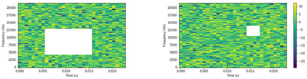
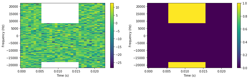
Example of TF representation of a complex signal, with binary masking
As for MaskedArray, TfData can be initialized from a 2D complex
nd-array with or without mask. Parameters stft_params and
signal_params are explicitly given if available. For a complex
signal, coefficients for both negative and positive frequencies are
handled and displayed
In [3]:
# Data ans mask for a complex signal (no symetry in TF)
tf_shape_complex = (tf_params['n_bins'], signal_params['len'] // tf_params['hop'])
mask_complex = np.zeros(tf_shape_complex)
mask_complex[int(0.2*tf_shape_complex[0]):int(0.6*tf_shape_complex[0]),
             int(0.25*tf_shape_complex[1]):int(0.7*tf_shape_complex[1])] = True
data_complex = np.random.randn(*tf_shape_complex) + 1j * np.random.randn(*tf_shape_complex)

# TF data
X = TfData(data=data_complex, mask=mask_complex, tf_params=tf_params, signal_params=signal_params)

plt.subplot(121)
X.plot_spectrogram()
plt.subplot(122)
X.plot_mask()
print(X)
========================
TF representation
------------------------
TF parameters
{'hop': 32, 'n_bins': 128, 'win_len': 64, 'win_name': 'hanning'}
------------------------
Signals parameters
{'len': 1024, 'fs': 44100}
------------------------
128 frequency bins
32 frames
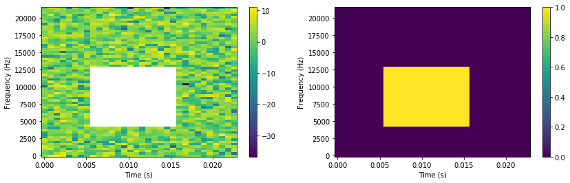
Example of TF representation of a real signal, with binary masking
For a real signal, only the non-negative frequencies area is handled due to Hermitian symetry.
In [4]:
# Data and mask for a real signal (Hermitian symetry in TF)
tf_shape_real = (tf_params['n_bins'] // 2 + 1, signal_params['len'] // tf_params['hop'])
mask_real = np.zeros(tf_shape_real)
mask_real[int(0.2*tf_shape_real[0]):int(0.6*tf_shape_real[0]),
          int(0.25*tf_shape_real[1]):int(0.7*tf_shape_real[1])] = True
data_real = np.random.randn(*tf_shape_real) + 1j * np.random.randn(*tf_shape_real)

# TF data
X = TfData(data=data_real, mask=mask_real, tf_params=tf_params, signal_params=signal_params)

plt.subplot(121)
X.plot_spectrogram()
plt.subplot(122)
X.plot_mask()
print(X)
========================
TF representation
------------------------
TF parameters
{'hop': 32, 'n_bins': 128, 'win_len': 64, 'win_name': 'hanning'}
------------------------
Signals parameters
{'len': 1024, 'fs': 44100}
------------------------
65 frequency bins
32 frames
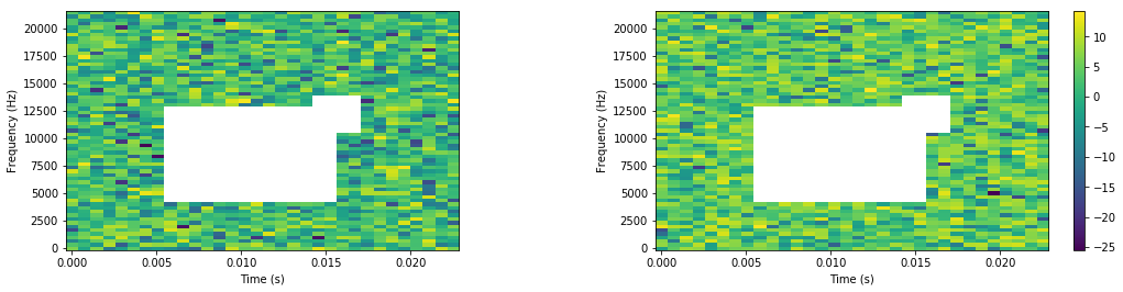
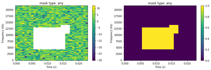
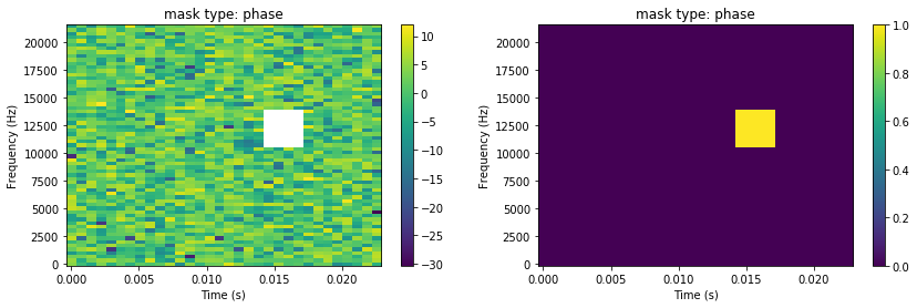
Example of TF representation with complex masking
With complex masking, two masks are handled: a mask for amplitudes and a mask for phases.
In [5]:
# Data and mask for a real signal (Hermitian symetry in TF)
tf_shape_real = (tf_params['n_bins'] // 2 + 1, signal_params['len'] // tf_params['hop'])
mask_mag = np.zeros(tf_shape_real)
mask_mag[int(0.2*tf_shape_real[0]):int(0.6*tf_shape_real[0]),
         int(0.25*tf_shape_real[1]):int(0.7*tf_shape_real[1])] = True
mask_phi = np.zeros(tf_shape_real)
mask_phi[int(0.5*tf_shape_real[0]):int(0.65*tf_shape_real[0]),
         int(0.65*tf_shape_real[1]):int(0.75*tf_shape_real[1])] = True
data_real = np.random.randn(*tf_shape_real) + 1j * np.random.randn(*tf_shape_real)

# TF data
X = TfData(data=data_real,
           mask_magnitude=mask_mag, mask_phase=mask_phi,
           tf_params=tf_params, signal_params=signal_params)
print(X)
========================
TF representation
------------------------
TF parameters
{'hop': 32, 'n_bins': 128, 'win_len': 64, 'win_name': 'hanning'}
------------------------
Signals parameters
{'len': 1024, 'fs': 44100}
------------------------
65 frequency bins
32 frames
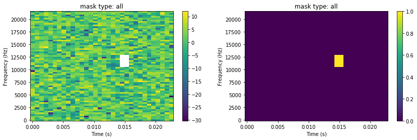
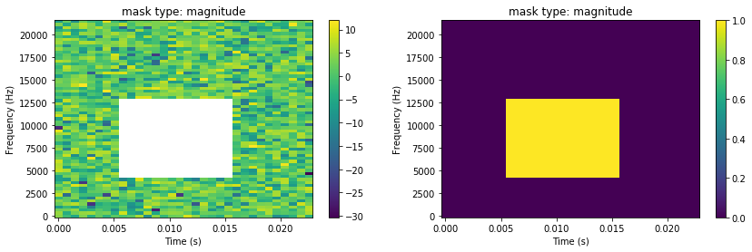
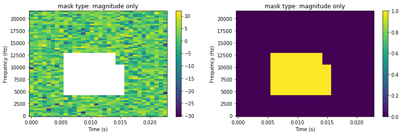
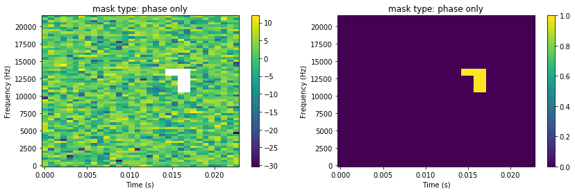
One may select one of the masks or a combination of them for display.
In [6]:
for mask_type in ['any', 'all', 'magnitude', 'phase', 'magnitude only', 'phase only']:
    plt.figure()
    plt.subplot(121)
    X.plot_spectrogram(mask_type=mask_type)
    plt.title('mask type: {}'.format(mask_type))
    plt.subplot(122)
    X.plot_mask(mask_type=mask_type)
    plt.title('mask type: {}'.format(mask_type))
Selecting a mask type can also be used to extract the related mask:
In [7]:
for mask_type in ['any', 'all', 'magnitude', 'phase', 'magnitude only', 'phase only']:
    mask = X.get_unknown_mask(mask_type)
    print('Ratio of "{}" unknown coefficients: {:.1%}'.format(mask_type, np.mean(mask)))
    mask = X.get_known_mask(mask_type)
    print('Ratio of "{}" known coefficients: {:.1%}'.format(mask_type, np.mean(mask)))
Ratio of "any" unknown coefficients: 18.8%
Ratio of "any" known coefficients: 99.3%
Ratio of "all" unknown coefficients: 0.7%
Ratio of "all" known coefficients: 81.2%
Ratio of "magnitude" unknown coefficients: 17.5%
Ratio of "magnitude" known coefficients: 82.5%
Ratio of "phase" unknown coefficients: 1.9%
Ratio of "phase" known coefficients: 98.1%
Ratio of "magnitude only" unknown coefficients: 16.8%
Ratio of "magnitude only" known coefficients: 1.2%
Ratio of "phase only" unknown coefficients: 1.2%
Ratio of "phase only" known coefficients: 16.8%
Other useful properties:
In [8]:
print('Number of frequencies: {}'.format(X.n_frequencies))
print('Number of frames: {}'.format(X.n_frames))
print('Start time of frames: {}'.format(X.start_times))
print('Center time of frames: {}'.format(X.mid_times))
print('End time of frames: {}'.format(X.end_times))
Number of frequencies: 65
Number of frames: 32
Start time of frames: [ -7.02947846e-04   2.26757370e-05   7.48299320e-04   1.47392290e-03
   2.19954649e-03   2.92517007e-03   3.65079365e-03   4.37641723e-03
   5.10204082e-03   5.82766440e-03   6.55328798e-03   7.27891156e-03
   8.00453515e-03   8.73015873e-03   9.45578231e-03   1.01814059e-02
   1.09070295e-02   1.16326531e-02   1.23582766e-02   1.30839002e-02
   1.38095238e-02   1.45351474e-02   1.52607710e-02   1.59863946e-02
   1.67120181e-02   1.74376417e-02   1.81632653e-02   1.88888889e-02
   1.96145125e-02   2.03401361e-02   2.10657596e-02   2.17913832e-02]
Center time of frames: [ 0.          0.00072562  0.00145125  0.00217687  0.00290249  0.00362812
  0.00435374  0.00507937  0.00580499  0.00653061  0.00725624  0.00798186
  0.00870748  0.00943311  0.01015873  0.01088435  0.01160998  0.0123356
  0.01306122  0.01378685  0.01451247  0.0152381   0.01596372  0.01668934
  0.01741497  0.01814059  0.01886621  0.01959184  0.02031746  0.02104308
  0.02176871  0.02249433]
End time of frames: [ 0.00070295  0.00142857  0.0021542   0.00287982  0.00360544  0.00433107
  0.00505669  0.00578231  0.00650794  0.00723356  0.00795918  0.00868481
  0.00941043  0.01013605  0.01086168  0.0115873   0.01231293  0.01303855
  0.01376417  0.0144898   0.01521542  0.01594104  0.01666667  0.01739229
  0.01811791  0.01884354  0.01956916  0.02029478  0.02102041  0.02174603
  0.02247166  0.02319728]
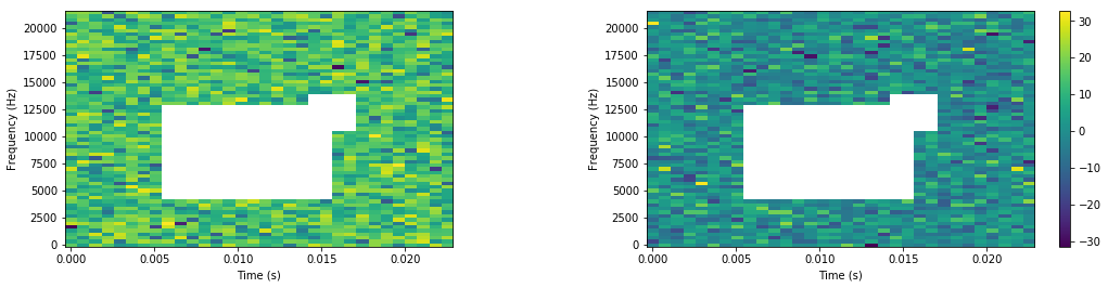
Current operations between two TfData objects are not recommended
since resulting operations on masks are not designed adequately:
In [9]:
mask1 = np.zeros(tf_shape_real)
mask1[int(0.2*tf_shape_real[0]):int(0.6*tf_shape_real[0]),
      int(0.25*tf_shape_real[1]):int(0.7*tf_shape_real[1])] = True
mask2 = np.zeros(tf_shape_real)
mask2[int(0.5*tf_shape_real[0]):int(0.65*tf_shape_real[0]),
      int(0.65*tf_shape_real[1]):int(0.75*tf_shape_real[1])] = True
data_real = np.random.randn(*tf_shape_real) + 1j * np.random.randn(*tf_shape_real)

# TF data
X1 = TfData(data=np.random.randn(*tf_shape_real) + 1j * np.random.randn(*tf_shape_real),
            mask=mask1, tf_params=tf_params, signal_params=signal_params)
X2 = TfData(data=np.random.randn(*tf_shape_real) + 1j * np.random.randn(*tf_shape_real),
            mask=mask2, tf_params=tf_params, signal_params=signal_params)

plt.figure()
plt.subplot(121)
X1.plot_spectrogram()
plt.subplot(122)
X2.plot_spectrogram()

plt.figure()
X3 = X1 + X2
X4 = X1 - X2
plt.subplot(121)
X3.plot_spectrogram()
plt.subplot(122)
X4.plot_spectrogram()

plt.figure()
X3 = X1 * X2
X4 = X1 / X2
plt.subplot(121)
X3.plot_spectrogram()
plt.subplot(122)
X4.plot_spectrogram()
pass