Time-frequency transforms : boundary effects
The examples below illustrate the effects of setting Stft-object flag zero_pad_full_sig to True (False) in order to avoid (obtain) a circular transform.
In [1]:
%pylab inline
import numpy as np
from madarrays import Waveform
from pyteuf import Stft
Populating the interactive namespace from numpy and matplotlib
Examples with isolated diracs
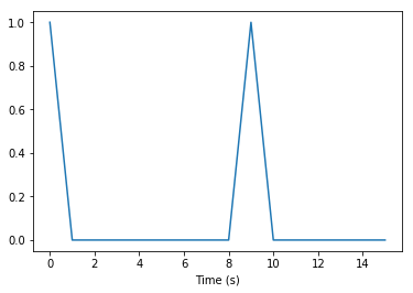
The signal with length 16 samples is composed of a dirac at initial time \(t=0\) for testing the boundary effects and another dirac time \(t=9\) for control.
In [2]:
signal_params_nopad = {'sig_len': 16, 'fs': 1}
x_nopad = Waveform(np.zeros(signal_params_nopad['sig_len']),
             fs = signal_params_nopad['fs'])
x_nopad[0] = x_nopad[9] = 1
print(x_nopad)
x_nopad.plot()
Waveform, fs=1Hz, length=16, dtype=float64, 0 missing entries (0.0%)
[ 1.  0.  0.  0.  0.  0.  0.  0.  0.  1.  0.  0.  0.  0.  0.  0.]
Out[2]:
[<matplotlib.lines.Line2D at 0x7f453b73b588>]
In [3]:
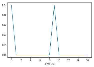
# Note that the signal length is increased by 1 in order
# to satisfy the `param_constraint='fix'` parameter of Stft (see tutorial on transform length)
signal_params_pad = {'sig_len': signal_params_nopad['sig_len']+1, 'fs': signal_params_nopad['fs']}
x_pad = Waveform(np.zeros(signal_params_pad['sig_len']),
                 fs = signal_params_pad['fs'])
x_pad[0] = x_pad[9] = 1
print(x_pad)
x_pad.plot()
Waveform, fs=1Hz, length=17, dtype=float64, 0 missing entries (0.0%)
[ 1.  0.  0.  0.  0.  0.  0.  0.  0.  1.  0.  0.  0.  0.  0.  0.  0.]
Out[3]:
[<matplotlib.lines.Line2D at 0x7f453b6dd4e0>]
Two similar Stft objects are defined, that differ only on the use of
additional zero-padding. By setting zero_pad_full_sig=False, no
additional zero-padding results in a circular transform. By setting
zero_pad_full_sig=True, zeros are added at the end of the signal in
an appropriate way such that the samples at the beginning and at the end
of the original signal are not appearing in the same frame (i.e., the
number of added zeros equals the window length minus one).
In [4]:
stft_params = {'hop': 1, 'n_bins': 4, 'win_name': 'hann', 'win_len': 4, 'param_constraint': 'fix'}
stft_nopad = Stft(zero_pad_full_sig=False, **stft_params)
print(stft_nopad)
stft_pad = Stft(zero_pad_full_sig=True, **stft_params)
print(stft_pad)
***************************** STFT *****************************
Specified analysis window: hann, 4 samples
Tight: False
Hop length: 1 samples
4 frequency bins
Convention: lp
param_constraint: fix
zero_pad_full_sig: False
****************************************************************
***************************** STFT *****************************
Specified analysis window: hann, 4 samples
Tight: False
Hop length: 1 samples
4 frequency bins
Convention: lp
param_constraint: fix
zero_pad_full_sig: True
****************************************************************
With the circular transform, the dirac at time \(t=0\) spread at times \(t=0\), \(t=1\) and \(t=15\) (i.e., at the last time step in the signal with length 16)
In [5]:
X_nopad = stft_nopad.apply(x_nopad)
print(X_nopad)
_ = X_nopad.plot_spectrogram(dynrange=100)
========================
TF representation
------------------------
TF parameters
{'hop': 1, 'n_bins': 4, 'win_name': 'hann', 'win_len': 4, 'win_array': None, 'win_type': 'analysis', 'is_tight': False, 'convention': 'lp', 'param_constraint': 'fix', 'zero_pad_full_sig': False}
------------------------
Signals parameters
{'fs': 1, 'sig_len': 16}
------------------------
3 frequency bins
16 frames
With additional zero-padding, the dirac at time \(t=0\) does not spread at \(t=15\) any more since the signal has been zero-padded to avoid circular effects (even if the transform is still circular). Energy is observed at time \(t=19\), i.e. in the area where the signal has been extended.
In [6]:
X_pad = stft_pad.apply(x_pad)
print(X_pad)
_ = X_pad.plot_spectrogram(dynrange=100)
========================
TF representation
------------------------
TF parameters
{'hop': 1, 'n_bins': 4, 'win_name': 'hann', 'win_len': 4, 'win_array': None, 'win_type': 'analysis', 'is_tight': False, 'convention': 'lp', 'param_constraint': 'fix', 'zero_pad_full_sig': True}
------------------------
Signals parameters
{'fs': 1, 'sig_len': 17}
------------------------
3 frequency bins
20 frames
Examples with diracs at boundaries
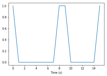
This example illustrate how the first and last samples are neighbors in the case of a circular transform. The signal is now composed of a dirac at each boundary, i.e., at times \(t=0\) and \(t=15\), as well as two neighboring diracs at times \(t=8\) and \(t=9\) for control.
In [7]:
x_nopad = Waveform(np.zeros(signal_params_nopad['sig_len']),
             fs = signal_params_nopad['fs'])
x_nopad[0] = x_nopad[-1] = x_nopad[8] = x_nopad[9] = 1
print(x_nopad)
x_nopad.plot()
Waveform, fs=1Hz, length=16, dtype=float64, 0 missing entries (0.0%)
[ 1.  0.  0.  0.  0.  0.  0.  0.  1.  1.  0.  0.  0.  0.  0.  1.]
Out[7]:
[<matplotlib.lines.Line2D at 0x7f453b563c18>]
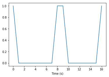
In [8]:
x_pad = Waveform(np.zeros(signal_params_pad['sig_len']),
             fs = signal_params_pad['fs'])
x_pad[0] = x_pad[-1] = x_pad[8] = x_pad[9] = 1
print(x_pad)
x_pad.plot()
Waveform, fs=1Hz, length=17, dtype=float64, 0 missing entries (0.0%)
[ 1.  0.  0.  0.  0.  0.  0.  0.  1.  1.  0.  0.  0.  0.  0.  0.  1.]
Out[8]:
[<matplotlib.lines.Line2D at 0x7f453b6560b8>]
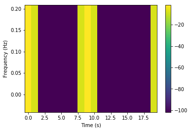
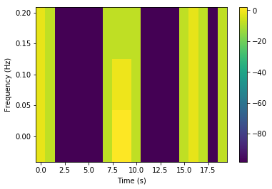
Without zero-padding, due to the circular transform, diracs influence each other and form a single area in the spectrogram, which is similar as the center area that contains two adjacent diracs.
In [9]:
stft_nopad.apply(x_nopad).plot_spectrogram(dynrange=100)
Out[9]:
array([[  1.76091259,  -7.7815125 , -98.23908741, -98.23908741,
        -98.23908741, -98.23908741, -98.23908741,  -7.7815125 ,
          1.76091259,   1.76091259,  -7.7815125 , -98.23908741,
        -98.23908741, -98.23908741,  -7.7815125 ,   1.76091259],
       [ -0.79181246,  -7.7815125 , -98.23908741, -98.23908741,
        -98.23908741, -98.23908741, -98.23908741,  -7.7815125 ,
         -0.79181246,  -0.79181246,  -7.7815125 , -98.23908741,
        -98.23908741, -98.23908741,  -7.7815125 ,  -0.79181246],
       [ -7.7815125 ,  -7.7815125 , -98.23908741, -98.23908741,
        -98.23908741, -98.23908741, -98.23908741,  -7.7815125 ,
         -7.7815125 ,  -7.7815125 ,  -7.7815125 , -98.23908741,
        -98.23908741, -98.23908741,  -7.7815125 ,  -7.7815125 ]])
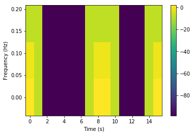
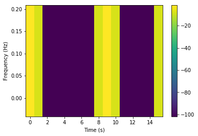
With additional zero-padding, the beginning and the end of the signal are separated with zeros so diracs are well resolved and do not appear as adjacent diracs.
In [10]:
_ = stft_pad.apply(x_pad).plot_spectrogram(dynrange=100)
Examples with a sinusoid
The signal is now a sinusoid and the length of the signal is a multiple of the period.
In [11]:
signal_params_nopad = {'sig_len': 32}
signal_params_nopad['fs'] = signal_params_nopad['sig_len'] - 1
signal_params_pad = {'sig_len': signal_params_nopad['sig_len'] + 1}
signal_params_pad['fs'] = signal_params_pad['sig_len'] - 1
f0 = 4 / signal_params_nopad['sig_len']
x_nopad = Waveform(np.sin(2 * np.pi * f0 * np.arange(signal_params_nopad['sig_len'])),
             fs = signal_params_nopad['fs'])
x_nopad.plot()
f0_pad = 4 / signal_params_pad['sig_len']
x_pad = Waveform(np.sin(2 * np.pi * f0_pad * np.arange(signal_params_pad['sig_len'])),
             fs = signal_params_pad['fs'])
x_pad.plot(linestyle='--')
Out[11]:
[<matplotlib.lines.Line2D at 0x7f453b4ae128>]
In [12]:
stft_params = {'hop': 1, 'n_bins': 16, 'win_name': 'hann', 'win_len': 16, 'param_constraint': 'fix'}
stft_nopad = Stft(zero_pad_full_sig=False, **stft_params)
print(stft_nopad)
stft_pad = Stft(zero_pad_full_sig=True, **stft_params)
print(stft_pad)
***************************** STFT *****************************
Specified analysis window: hann, 16 samples
Tight: False
Hop length: 1 samples
16 frequency bins
Convention: lp
param_constraint: fix
zero_pad_full_sig: False
****************************************************************
***************************** STFT *****************************
Specified analysis window: hann, 16 samples
Tight: False
Hop length: 1 samples
16 frequency bins
Convention: lp
param_constraint: fix
zero_pad_full_sig: True
****************************************************************
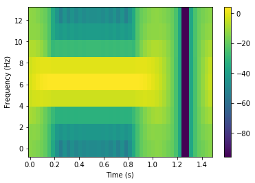
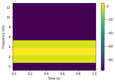
Periodic tranform: as the length of the signal is a multiple of the period, the circular transform coefficients are constant over time.
In [13]:
X_nopad = stft_nopad.apply(x_nopad)
print(X_nopad)
_ = X_nopad.plot_spectrogram(dynrange=100)
========================
TF representation
------------------------
TF parameters
{'hop': 1, 'n_bins': 16, 'win_name': 'hann', 'win_len': 16, 'win_array': None, 'win_type': 'analysis', 'is_tight': False, 'convention': 'lp', 'param_constraint': 'fix', 'zero_pad_full_sig': False}
------------------------
Signals parameters
{'fs': 31, 'sig_len': 32}
------------------------
9 frequency bins
32 frames
With additional zeros to avoid circular effects, transients appear at boundaries.
In [14]:
X_pad = stft_pad.apply(x_pad)
print(X_pad)
_ = X_pad.plot_spectrogram(dynrange=100)
========================
TF representation
------------------------
TF parameters
{'hop': 1, 'n_bins': 16, 'win_name': 'hann', 'win_len': 16, 'win_array': None, 'win_type': 'analysis', 'is_tight': False, 'convention': 'lp', 'param_constraint': 'fix', 'zero_pad_full_sig': True}
------------------------
Signals parameters
{'fs': 32, 'sig_len': 33}
------------------------
9 frequency bins
48 frames
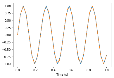
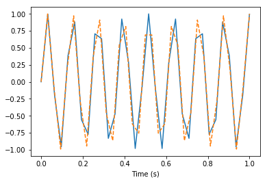
Now, if the period is not a divisor of the length of the signal:
In [15]:
signal_params_nopad = {'sig_len': 32}
signal_params_nopad['fs'] = signal_params_nopad['sig_len'] - 1
signal_params_pad = {'sig_len': signal_params_nopad['sig_len'] + 1}
signal_params_pad['fs'] = signal_params_pad['sig_len'] - 1
f0 = 8.5 / signal_params_nopad['sig_len']
x_nopad = Waveform(np.sin(2 * np.pi * f0 * np.arange(signal_params_nopad['sig_len'])),
             fs = signal_params_nopad['fs'])
x_nopad.plot()
f0_pad = 8.5 / signal_params_pad['sig_len']
x_pad = Waveform(np.sin(2 * np.pi * f0_pad * np.arange(signal_params_pad['sig_len'])),
             fs = signal_params_pad['fs'])
x_pad.plot(linestyle='--')
Out[15]:
[<matplotlib.lines.Line2D at 0x7f453b27d860>]
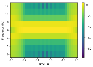
Some boundary effects appear in the case without zero-padding due to the discontinuity between the end and the beginning of the signal:
In [16]:
X_nopad = stft_nopad.apply(x_nopad)
print(X_nopad)
_ = X_nopad.plot_spectrogram(dynrange=100)
========================
TF representation
------------------------
TF parameters
{'hop': 1, 'n_bins': 16, 'win_name': 'hann', 'win_len': 16, 'win_array': None, 'win_type': 'analysis', 'is_tight': False, 'convention': 'lp', 'param_constraint': 'fix', 'zero_pad_full_sig': False}
------------------------
Signals parameters
{'fs': 31, 'sig_len': 32}
------------------------
9 frequency bins
32 frames
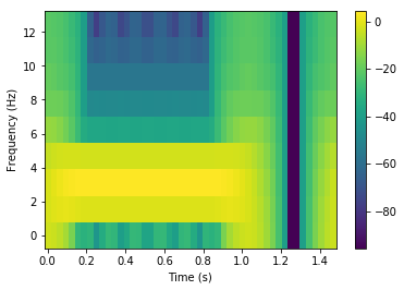
Some boundary effects also appear in the case with zero-padding due to the discontinuity with the added zeros:
In [17]:
X_pad = stft_pad.apply(x_pad)
print(X_pad)
_ = X_pad.plot_spectrogram(dynrange=100)
========================
TF representation
------------------------
TF parameters
{'hop': 1, 'n_bins': 16, 'win_name': 'hann', 'win_len': 16, 'win_array': None, 'win_type': 'analysis', 'is_tight': False, 'convention': 'lp', 'param_constraint': 'fix', 'zero_pad_full_sig': True}
------------------------
Signals parameters
{'fs': 32, 'sig_len': 33}
------------------------
9 frequency bins
48 frames