Tutorial for package yafe

This tutorial shows the basics for:

• designing an experiment by specifying some data, a problem, a solver, performance measures and related parameters;
• running an experiment, i.e. running all related tasks;
• collecting and analyzing the results of an experiments;
• updating an experiment by adding tasks and running them;
• dealing with multiple instances of an experiment, e.g. to compare solvers;
• understanding yafe in more details for debugging or developing more in depth: looking at one specific task, using functions instead of classes, understanding yafe’s internal mechanisms.

In order to illustrate how to use yafe, a simple experiment is implemented: from signals synthesized from a sinusoidal model with several possible frequencies, generate denoising problem by adding Gaussian noise with several signal-to-noise ratio (SNR) levels, solve each problem using a low-pass filter with a filter length parameter and compute the performance in terms of signal-to-distortion ratio (SDR).

%load_ext autoreload
%autoreload 2

%matplotlib inline

import yafe
import numpy as np
import matplotlib.pyplot as plt
try:
    # The xarray package is optional, it may enhance how to handle results
    import xarray
except:
    xarray = None

import tempfile
# For this tutorial, we will store the data of our experiments in a temporary directory
temp_data_path = tempfile.mkdtemp(prefix='yafe_')

Design an experiment

An experiment is based on:

• a workflow composed of four blocks: data access, problem generation, solver, performance measures
• a set of parameters for each block, whom cartesian product will define the set of all tasks

Designing an experiment consists in defining each of those blocks and the set of related parameters.

Let us examine a simple signal denoising example.

Define access to data

Data access should be performed by a function that ouputs the data in a dictionary, depending on some parameters passed as arguments. Data parameters must be given in a dictionary whose keys match the parameter names and whose values are the ranges of each parameter, given as lists or 1D ndarrays.

In this example, the generated data is a sinusoid with two parameters, length and frequency. The length takes only one value while the frequency ranges from 0.01 to 0.1.

def get_sine_data(f0, signal_len=1000):
    return {'signal': np.sin(2*np.pi*f0*np.arange(signal_len))}
data_params = {'f0': np.arange(0.01, 0.1, 0.01), 'signal_len': [1000]}

Define problem generation (using classes)

A simple way to define problem generation is to create a class and to follow four rules:

• the inputs of the __init__ method are the parameters of the problem
• the parameters of the __call__ method match the keys of the dictionary obtained from the data access function get_data
• the output of the __call__ method is a dictionary containing the problem data for the solver

In this example, noise is added to the input signal, with a signal-to-noise ratio given as a problem parameter. An optional __str__ is defined here.

class SimpleDenoisingProblem:
    def __init__(self, snr_db):
        self.snr_db = snr_db

    def __call__(self, signal):
        random_state = np.random.RandomState(0)
        noise = random_state.randn(*signal.shape)
        observation = signal + 10 ** (-self.snr_db / 20) * noise / np.linalg.norm(noise) * np.linalg.norm(signal)
        problem_data = {'observation': observation}
        solution_data = {'signal': signal}
        return (problem_data, solution_data)

    def __str__(self):
        return 'SimpleDenoisingProblem(snr_db={})'.format(self.snr_db)

problem_params = {'snr_db': [-10, 0, 30]}

Define solvers (using classes)

Solvers can be defined in a similar way as problems, by creating a class and by following four rules:

• the parameters of the solver are passed to the __init__ method
• the parameters of the __call__ method match the keys of the dictionary obtained from the problem generation method __call__
• the output of the __call__ method is a dictionary containing the solution estimated by the solver.

In this example, the problem is solved by low-pass filtering the noisy observation, the filter length being the unique solver parameter. An optional __str__ is defined here.

class SmoothingSolver:
    def __init__(self, filter_len):
        self.filter_len = filter_len

    def __call__(self, observation):
        smoothing_filter = np.hamming(self.filter_len)
        smoothing_filter /= np.sum(smoothing_filter)
        return {'reconstruction': np.convolve(observation, smoothing_filter, mode='same')}

    def __str__(self):
        return 'SmoothingSolver(filter_len={})'.format(self.filter_len)

solver_params = {'filter_len': 2**np.arange(6, step=2)}

Note that one may also define problem and solvers using functions instead of classes, as described in section Alternate way using functions.

Define measures

Several performance measures may be calculated from the estimated solution, using other data like the original data, the problem data, or parameters of the data, problem or solver.

These performance measures must be computed within a function as follows:

• its arguments should be dictionaries source_data, problem_data, solution_data and solved_data, as returned by the data access function, the __call__ methods of problem generation class and the __call__ methods of solver class, respectively; an additional argument task is a dictionary that contains the data, problem and solver parameters;
• its output is a dictionary whose keys and values are the names and values of the various performance measures.

In this example, the signal-to-distortion ratio, the euclidian distance and the infinite distance are computed between the estimated solution and the noiseless reference signal.

def measure(solution_data, solved_data, task_params=None, source_data=None, problem_data=None):
    euclidian_distance = np.linalg.norm(solution_data['signal']-solved_data['reconstruction'])
    sdr = 20 * np.log10(np.linalg.norm(solution_data['signal']) / euclidian_distance)
    inf_distance = np.linalg.norm(solution_data['signal']-solved_data['reconstruction'], ord=np.inf)
    return {'sdr': sdr, 'euclidian_distance': euclidian_distance, 'inf_distance': inf_distance}

Create the experiment

All the components being defined, one can simply create an experiment as an instance of the Experiment class, by passing a name and each component to the constructor.

my_first_exp = yafe.Experiment(name='My first experiment',
                               get_data=get_sine_data,
                               get_problem=SimpleDenoisingProblem,
                               get_solver=SmoothingSolver,
                               measure=measure,
                               force_reset=True,
                               data_path=temp_data_path,
                               log_to_file=False,
                               log_to_console=False)

Add all parameters as tasks

Then all the parameters’ ranges are passed to the add_tasks method.

my_first_exp.add_tasks(data_params=data_params, problem_params=problem_params, solver_params=solver_params)
print(my_first_exp)

Name: My first experiment
Data stored in: /tmp/yafe_futffym1/My first experiment
Not storing any debug information
Data provider: <function get_sine_data at 0x7f92a47dac80>
Problem provider : <class '__main__.SimpleDenoisingProblem'>
Solver provider: <class '__main__.SmoothingSolver'>
Measure: <function measure at 0x7f92a47ec9d8>

Parameters:
 Data parameters:
  f0: [0.01, 0.02, 0.029999999999999999, 0.040000000000000001, 0.050000000000000003, 0.060000000000000005, 0.069999999999999993, 0.080000000000000002, 0.089999999999999997]
  signal_len: [1000]
 Problem parameters:
  snr_db: [-10, 0, 30]
 Solver parameters:
  filter_len: [1, 4, 16]

Status:
Number of tasks: 0
Number of finished tasks: 0
Number of failed tasks: 0
Number of pending tasks: 0

Run an experiment

Running an experiment consists in:

• generating tasks from the experiment parameters
• executing all pending tasks
• collecting all the task results

At this point, no task appear:

my_first_exp.display_status()

Number of tasks: 0
Number of finished tasks: 0
Number of failed tasks: 0
Number of pending tasks: 0

One must call the generate_tasks method, which will set up the internal mechanisms to create tasks, the set of tasks being the cartesian product between all parameter ranges in the experiment.

my_first_exp.generate_tasks()

my_first_exp.display_status()

Number of tasks: 81
Number of finished tasks: 0
Number of failed tasks: 0
Number of pending tasks: 81

One can see the total number of tasks, which equals the product between the size of all parameter ranges in the experiment:

print(np.product([np.array(v).size
                  for params in (data_params, problem_params, solver_params)
                  for v in params.values()]))

81

One may run a specific task from its id:

my_first_exp.run_task_by_id(idt=5)
my_first_exp.display_status()

Number of tasks: 81
Number of finished tasks: 1
Number of failed tasks: 0
Number of pending tasks: 80

This may usefull to check whether a task is running successfully, to run a specific task within a job on a computer cluster.

One may also run all pending tasks:

my_first_exp.launch_experiment()

my_first_exp.display_status()

Number of tasks: 81
Number of finished tasks: 81
Number of failed tasks: 0
Number of pending tasks: 0

Results from all tasks needs to be collected and gathered in a unique structure before being analyzed.

my_first_exp.collect_results()

Exploit results

Results are stored in a hypercube whose axes are the parameters of the experiment, with an additional axis containing the performance measures. After collecting results, one may load them in an ndarray together with the labels and values of the related axes:

results, axes_labels, axes_values = my_first_exp.load_results()
print(results.shape, results.dtype)
print(axes_labels)
print(axes_values)
# Let us display one value:
print('Euclidian distance value for paramenters f0=0.04, signal length=1000, SNR=30 and filter length=1:',
      results[3, 0, 2, 0, 1])

(9, 1, 3, 3, 3) float64
['data_f0' 'data_signal_len' 'problem_snr_db' 'solver_filter_len' 'measure']
[array([ 0.01,  0.02,  0.03,  0.04,  0.05,  0.06,  0.07,  0.08,  0.09])
 array([1000]) array([-10,   0,  30]) array([ 1,  4, 16])
 array(['sdr', 'euclidian_distance', 'inf_distance'], dtype=object)]
Euclidian distance value for paramenters f0=0.04, signal length=1000, SNR=30 and filter length=1: 0.707106781187

One may then analyze and display the results.

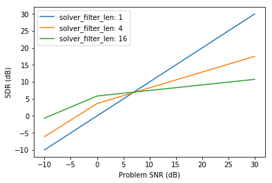
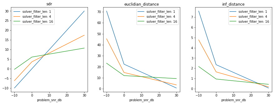
Here, performance measures are average along the data axes, and the resulting averaged SDR measure is displayed as a function of the problem SNR for each filter length:

# Compute average results w.r.t. all data (axis 0 and 1)
mean_results = np.mean(results, axis=(0, 1))

# For each solver parameter (axis 3), plot SDR (axis 4, first element) as a function of the problem SNR (axis 2)
for i_solver_param, solver_param in enumerate(axes_values[3]):
    plt.plot(axes_values[2],
             mean_results[:, i_solver_param, 0],
             label='{}: {}'.format('solver_filter_len', solver_param))
plt.xlabel('Problem SNR (dB)')
plt.ylabel('SDR (dB)')
plt.legend()
pass

One can note that handling such multidimensional arrays and their multiple axes is likely to be confusing and is prone to dissimulate errors. A more convenient and reliable way is to handle an DataArray object, from the optional package xarray:

if xarray:
    xresults = my_first_exp.load_results(array_type='xarray')
    print(xresults.shape)
    print(xresults.coords)
    # Let us display one value:
    print('Euclidian distance value for paramenters f0=0.04, signal length=1000, SNR=30 and filter length=1:')
    print(xresults.sel(data_f0=0.04,
                       data_signal_len=1000,
                       problem_snr_db=30,
                       solver_filter_len=1,
                       measure='euclidian_distance'))

(9, 1, 3, 3, 3)
Coordinates:
  * data_f0            (data_f0) float64 0.01 0.02 0.03 0.04 0.05 0.06 0.07 ...
  * data_signal_len    (data_signal_len) int64 1000
  * problem_snr_db     (problem_snr_db) int64 -10 0 30
  * solver_filter_len  (solver_filter_len) int64 1 4 16
  * measure            (measure) object 'sdr' 'euclidian_distance' ...
Euclidian distance value for paramenters f0=0.04, signal length=1000, SNR=30 and filter length=1:
<xarray.DataArray ()>
array(0.7071067811865467)
Coordinates:
    data_f0            float64 0.04
    data_signal_len    int64 1000
    problem_snr_db     int64 30
    solver_filter_len  int64 1
    measure            <U18 'euclidian_distance'

if xarray:
    # Compute average results w.r.t. all data
    mean_results = xresults.mean(['data_f0', 'data_signal_len'])

    # For each solver parameter, plot SDR as a function of the problem SNR
    for solver_param in mean_results['solver_filter_len'].values:
        plt.plot(mean_results['problem_snr_db'].values,
                 mean_results.sel(solver_filter_len=solver_param, measure='sdr'),
                 label='{}: {}'.format('solver_filter_len', solver_param))
        plt.legend()
        plt.xlabel('Problem SNR (dB)')
        plt.ylabel('SDR (dB)')

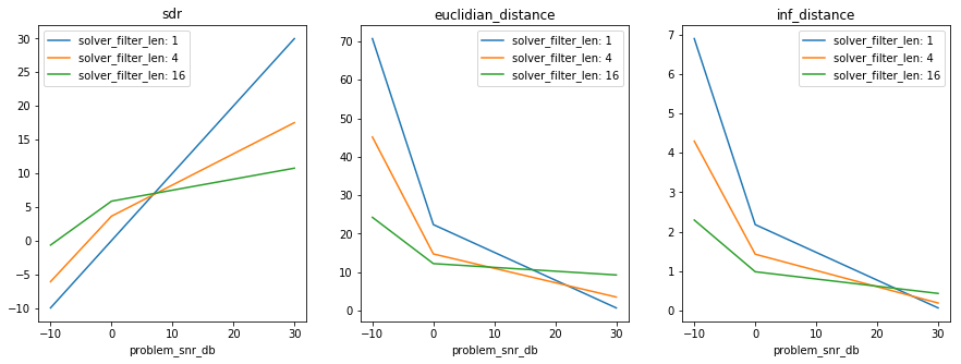
Here is an extended plot of the results, which is provided equivalently in the numpy and xarray result format.

def plot_results(results, axes_labels, axes_values):
    fig = plt.gcf()
    axes = fig.subplots(1, results.shape[4])
    mean_results = np.mean(results, axis=(0, 1))  # Average w.r.t. input data
    for i_meas in range(results.shape[4]):
        for i_solver_param, solver_param in enumerate(axes_values[3]):
            axes[i_meas].plot(axes_values[2],
                              mean_results[:, i_solver_param, i_meas],
                              label='{}: {}'.format(axes_labels[3], solver_param))
        axes[i_meas].set_xlabel('problem_snr_db')
        axes[i_meas].set_title(axes_values[4][i_meas])
        axes[i_meas].legend()

if xarray:
    def plot_xresults(xresults):
        fig = plt.gcf()
        abscissa = 'problem_snr_db'
        k_solver_param = [s for s in xresults.dims if s.startswith('solver_')][0]  # Find solver parameter key
        fig = plt.gcf()
        axes = fig.subplots(1, xresults['measure'].values.size)
        mean_results = xresults.mean(['data_f0', 'data_signal_len'])  # Average w.r.t. input data
        for i_meas, k_meas in enumerate(mean_results['measure'].values):
            for solver_param in mean_results[k_solver_param].values:
                sel_dict = {'measure': k_meas, k_solver_param: solver_param}  # Use a dict to select results
                axes[i_meas].plot(mean_results[abscissa].values,
                                  mean_results.sel(**sel_dict),
                                  label='{}: {}'.format(k_solver_param, solver_param))
            axes[i_meas].set_xlabel(abscissa)
            axes[i_meas].set_title(k_meas)
            axes[i_meas].legend()

plt.figure(figsize=(15, 5))
plot_results(results, axes_labels, axes_values)

if xarray:
    plt.figure(figsize=(15, 5))
    plot_xresults(xresults)

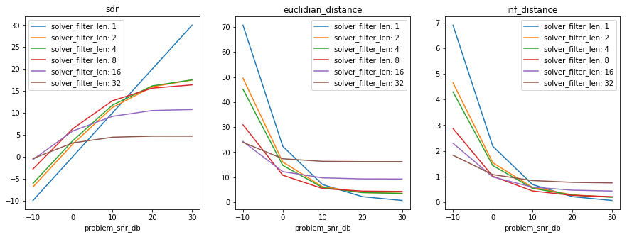
Add news tasks

Adding new task is perfomed by calling add_tasks again with additional parameters. It will cause the extension of the cartesian product as if all the parameters had been given together. Tasks that were previously completed will not be executed again.

additional_snr_db = [10, 20]
additional_filter_len = 2**np.arange(6)
my_first_exp.add_tasks(problem_params={'snr_db': additional_snr_db}, data_params=dict(),
                 solver_params={'filter_len': additional_filter_len})
my_first_exp.generate_tasks()
my_first_exp.display_status()

Number of tasks: 270
Number of finished tasks: 81
Number of failed tasks: 0
Number of pending tasks: 189

my_first_exp.launch_experiment()

my_first_exp.collect_results()

results, axes_labels, axes_values = my_first_exp.load_results()
plt.figure(figsize=(15, 5))
plot_results(results, axes_labels, axes_values)

if xarray:
    xresults = my_first_exp.load_results(array_type='xarray')
    plt.figure(figsize=(15, 5))
    plot_xresults(xresults)

Use several solvers

One may define several solvers to address the same problem and compare various approaches.

For instance, let us create a solver that uses median filtering, with the radius of the local filter as parameter:

class MedianSolver():
    def __init__(self, radius):
        self.radius = radius

    def __call__(self, observation):
        reconstruction = np.zeros_like(observation)
        for i in range(observation.size):
            i_start = max(0, i - self.radius)
            i_end = min(observation.size, i + self.radius + 1)
            reconstruction[i] = np.median(observation[i_start:i_end])
        return {'reconstruction': reconstruction}

    def __str__(self):
        return 'MedianSolver(radius={})'.format(self.radius)

median_solver_params = {'radius': [0, 1, 5, 10]}

One must create a new instance of the Experiment for each solver, using the same parameters, functions and classes for the data, problem and performance measures (creating a new instance is needed since the solvers are not sharing the same parameter space):

median_solver_exp = yafe.Experiment(name='Median solver experiment',
                                    get_data=get_sine_data,
                                    get_problem=SimpleDenoisingProblem,
                                    get_solver=MedianSolver,
                                    measure=measure,
                                    force_reset=True,
                                    data_path=temp_data_path,
                                    log_to_file=False,
                                    log_to_console=False)
median_solver_exp.add_tasks(data_params=data_params, problem_params=problem_params, solver_params=median_solver_params)
median_solver_exp.add_tasks(problem_params={'snr_db': additional_snr_db}, data_params=dict(), solver_params=dict())
median_solver_exp.generate_tasks()
median_solver_exp.display_status()

Number of tasks: 180
Number of finished tasks: 0
Number of failed tasks: 0
Number of pending tasks: 180

median_solver_exp.launch_experiment()

median_solver_exp.collect_results()

if xarray:
    xresults = median_solver_exp.load_results(array_type='xarray')
    plt.figure(figsize=(15, 5))
    plot_xresults(xresults)
else:
    results, axes_labels, axes_values = median_solver_exp.load_results()
    plt.figure(figsize=(15, 5))
    plot_results(results, axes_labels, axes_values)

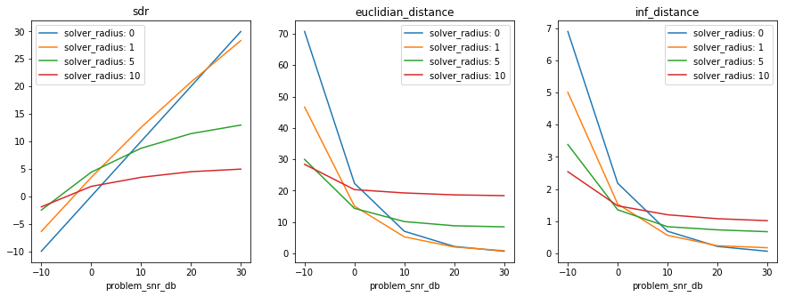
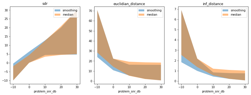
One can then compare the solvers, with results in either ndarray or xarray format:

def compare_solvers_and_plot_results(smooth_results, smooth_axes_labels, smooth_axes_values,
                                     median_results, median_axes_labels, median_axes_values):
    """ Compare ndarray-format results between two solvers,

    The results are assumed to be structured as follows:
    * both smooth_results and median_results should have similar structures,
      including order of axes labels and axes values
    * data parameters are on axes 0 and 1
    * problem parameter SNR is on axis 2
    * solver parameter is on axis 3
    * performance measure is on axis 4
    """
    fig = plt.gcf()
    axes = fig.subplots(1, smooth_results.shape[-1])
    for results, axes_labels, axes_values, name in [
        (smooth_results, smooth_axes_labels, smooth_axes_values, 'smoothing'),
        (median_results, median_axes_labels, median_axes_values, 'median')]:
        mean_results = np.mean(results, axis=(0, 1))  # Average w.r.t. input data
        for i_meas in range(results.shape[-1]):  # One measure per subplot
            # Fill an area between min and max values w.r.t. solver parameters
            axes[i_meas].fill_between(axes_values[2],
                                      np.min(mean_results[:, :, i_meas], axis=1),
                                      np.max(mean_results[:, :, i_meas], axis=1),
                                      alpha=0.5,
                                      label=name)
            axes[i_meas].set_xlabel(axes_labels[2])
            axes[i_meas].set_title(axes_values[-1][i_meas])
            axes[i_meas].legend()

if xarray:
    def compare_solvers_and_plot_xresults(smooth_xresults, median_xresults):
        """ Compare xarray-format results between two solvers """
        fig = plt.gcf()
        abscissa = 'problem_snr_db'
        axes = fig.subplots(1, smooth_xresults['measure'].values.size)
        for xresults, name in [(smooth_xresults, 'smoothing'), (median_xresults, 'median')]:
            k_solver_param = [s for s in xresults.dims if s.startswith('solver_')][0]  # Find solver parameter key
            mean_results = xresults.mean(['data_f0', 'data_signal_len'])  # Average w.r.t. input data
            for i_meas, k_meas in enumerate(mean_results['measure'].values):  # One measure per subplot
                # Fill an area between min and max values w.r.t. solver parameters
                axes[i_meas].fill_between(mean_results[abscissa].values,
                                          mean_results.sel(measure=k_meas).min(k_solver_param),
                                          mean_results.sel(measure=k_meas).max(k_solver_param),
                                          alpha=0.5,
                                          label=name)
                axes[i_meas].set_xlabel(abscissa)
                axes[i_meas].set_title(k_meas)
                axes[i_meas].legend()

Note that structures getting more complex, one may prefer to handle xarray objects for clarity and error-free purposes.

smooth_results, smooth_axes_labels, smooth_axes_values = my_first_exp.load_results()
median_results, median_axes_labels, median_axes_values = median_solver_exp.load_results()
fig = plt.figure(figsize=(15, 5))
compare_solvers_and_plot_results(
    smooth_results, smooth_axes_labels, smooth_axes_values,
    median_results, median_axes_labels, median_axes_values)

if xarray:
    smooth_xresults = my_first_exp.load_results(array_type='xarray')
    median_xresults = median_solver_exp.load_results(array_type='xarray')
    fig = plt.figure(figsize=(15, 5))
    compare_solvers_and_plot_xresults(smooth_xresults, median_xresults)

Look at one specific task

Let us detail how to handle one specific task.

From a task id

In order to look at a particular task from its id, get all available data using method get_task_data_by_id:

idt = 27
task_data = my_first_exp.get_task_data_by_id(idt=idt)
print(task_data.keys())

dict_keys(['id_task', 'task_params', 'source_data', 'problem_data', 'solution_data', 'solved_data', 'result'])

One may then recompute easily some part of the process:

# Get source data
source_data = my_first_exp.get_data(**task_data['task_params']['data_params'])
print(task_data['task_params']['data_params'])

# Get problem, problem data and that it equals what was computed previously
problem = my_first_exp.get_problem(**task_data['task_params']['problem_params'])
print(problem)
problem_data, solution_data = problem(**source_data)

# Get solver, compute solved data
solver = my_first_exp.get_solver(**task_data['task_params']['solver_params'])
print(solver)
solved_data = solver(**problem_data)

# Compute performane measures
results = my_first_exp.measure(solution_data=solution_data, solved_data=solved_data)
print('Performance measures:', results)

# Compare all generated data to what was computed previously
print('Source data match:', np.all(source_data['signal'] == task_data['source_data']['signal']))
print('Problem data match:', np.all(problem_data['observation'] == task_data['problem_data']['observation']))
print('Solved data match:', np.all(solved_data['reconstruction'] == task_data['solved_data']['reconstruction']))
print('Performance measure match:',
      np.all([np.all(results[k_measure] == task_data['result'][k_measure])
             for k_measure in results.keys()]))

{'f0': 0.040000000000000001, 'signal_len': 1000}
SimpleDenoisingProblem(snr_db=-10)
SmoothingSolver(filter_len=1)
Performance measures: {'sdr': -10.0, 'euclidian_distance': 70.710678118654684, 'inf_distance': 6.8936228098787975}
Source data match: True
Problem data match: True
Solved data match: True
Performance measure match: True

From task parameters

In order to look at a particular task from its parameters, get all available data using method get_task_data_by_id, using data_*, problem_*, solver_* to denote parameters of the data, problem and solver providers respectively, replacing * by the name of the parameter.

task_data = my_first_exp.get_task_data_by_params(data_params={'f0': 0.05, 'signal_len': 1000},
                                                 problem_params={'snr_db': 0},
                                                 solver_params={'filter_len': 4})
print('Task ID:', task_data['id_task'])

Task ID: 40

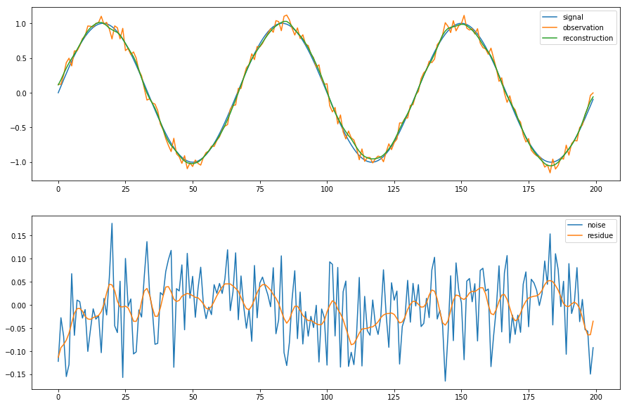
Specifying arbitrary parameter values

Here, parameter values are not in the parameter ranges of the experiment

data_params={'f0': 0.015, 'signal_len': 200}
problem_params={'snr_db': 20}
solver_params={'filter_len': 9}

# Get source data
source_data = my_first_exp.get_data(**data_params)

# Get problem, problem data and that it equals what was computed previously
problem = my_first_exp.get_problem(**problem_params)
print(problem)
problem_data, solution_data = problem(**source_data)

# Get solver, compute solved data
solver = my_first_exp.get_solver(**solver_params)
print(solver)
solved_data = solver(**problem_data)

# Compute performane measures
results = my_first_exp.measure(solution_data= solution_data, solved_data=solved_data)
print('Performance measures:', results)

SimpleDenoisingProblem(snr_db=20)
SmoothingSolver(filter_len=9)
Performance measures: {'sdr': 26.807450661453153, 'euclidian_distance': 0.45669627246336086, 'inf_distance': 0.11312791438321826}

fig = plt.figure(figsize=(15,10))
axes = fig.subplots(2, 1)
axes[0].plot(source_data['signal'], label='signal')
axes[0].plot(problem_data['observation'], label='observation')
axes[0].plot(solved_data['reconstruction'], label='reconstruction')
axes[0].legend()
axes[1].plot(source_data['signal']-problem_data['observation'], label='noise')
axes[1].plot(source_data['signal']-solved_data['reconstruction'], label='residue')
axes[1].legend()
pass

An alternate way using functions

When designing a problem and a solver, one may want to use functions only instead of classes. Here is the variant of the first experiment using functions only

data_params = {'f0': np.arange(0.01, 0.1, 0.01), 'signal_len': [1000]}
def add_noise_to_signal(signal, snr_db):
    noise = np.random.randn(*signal.shape)
    observation = signal + 10 ** (-snr_db / 20) * noise / np.linalg.norm(noise) * np.linalg.norm(signal)
    return observation

def get_problem(snr_db):
    def generate_problem(signal):
        problem_data = {'observation': add_noise_to_signal(signal, snr_db)}
        solution_data = {'signal': signal}
        return (problem_data, solution_data)
    return generate_problem

problem_params = {'snr_db': [-10, 0, 30]}

def denoise_with_smooth_filter(observation, filter_len):
    filter = np.hamming(filter_len)
    filter /= np.sum(filter)
    return np.convolve(observation, filter, mode='same')

def get_solver(filter_len):
    def solve_problem(observation):
        return {'reconstruction': denoise_with_smooth_filter(observation, filter_len)}
    return solve_problem

solver_params = {'filter_len': 2**np.arange(6, step=2)}

variant_exp = yafe.Experiment(name='Variant of first experiment',
                              get_data=get_sine_data,
                              get_problem=get_problem,
                              get_solver=get_solver,
                              measure=measure,
                              force_reset=True,
                              data_path=temp_data_path,
                              log_to_file=False,
                              log_to_console=False)
variant_exp.add_tasks(data_params=data_params, problem_params=problem_params, solver_params=solver_params)
print(variant_exp._schema)
variant_exp.generate_tasks()
variant_exp.launch_experiment()
variant_exp.collect_results()

{('data', 'f0'): [0.01, 0.02, 0.029999999999999999, 0.040000000000000001, 0.050000000000000003, 0.060000000000000005, 0.069999999999999993, 0.080000000000000002, 0.089999999999999997], ('data', 'signal_len'): [1000], ('problem', 'snr_db'): [-10, 0, 30], ('solver', 'filter_len'): [1, 4, 16]}

plt.figure(figsize=(15, 5))
if xarray:
    xresults = variant_exp.load_results(array_type='xarray')
    plt.figure(figsize=(15, 5))
    plot_xresults(xresults)
else:
    results, axes_labels, axes_values = variant_exp.load_results()
    plot_results(results, axes_labels, axes_values)

<matplotlib.figure.Figure at 0x7f92a2cf2710>

Internal mechanisms

Here are some details about how an experiment is handled internally. This should not be needed for the general user but may help in some cases (debugging, extending yafe, and so on).

Experiment._schema

Attribute _schema is a dictionary where all the experiment parameters are stored. Keys are tuples with two elements: the first one denotes the block related to the parameter ('data', 'problem' or 'solver'); the second one is the parameter name defined by the user. Attribute _schema should not be modified by the user in order to preserve the integrity of the Experiment object and related data.

my_first_exp._schema

{('data', 'f0'): [0.01,
  0.02,
  0.029999999999999999,
  0.040000000000000001,
  0.050000000000000003,
  0.060000000000000005,
  0.069999999999999993,
  0.080000000000000002,
  0.089999999999999997],
 ('data', 'signal_len'): [1000],
 ('problem', 'snr_db'): [-10, 0, 10, 20, 30],
 ('solver', 'filter_len'): [1, 2, 4, 8, 16, 32]}

Task numbering

Task IDs are assigned to new tasks once for all when generating tasks (Experiment.generate_tasks). The method looks at the IDs already assigned to existing tasks and assign available IDs to new tasks. As a consequence, task IDs are dependent on the sequence of task creations and does not only depends on the combination of parameters related to the task. This make it easier the management of task IDs when adding new tasks. This also implies that finding the one-to-one matching between task IDs and parameters requires to parse all task data from their ID and to check the parameters of each task. This is time consuming but only happens when generating tasks, collecting results and checking the status of the Experiment.

Internal data files

Experiments and related tasks are relying on files where parameters, intermediate data and final results are stored:

• All files are stored in a folder whose name matches that of the experiment, located either in the path passed using the parameter data_path when creating the Experiment, or in the data path defined in the user-defined yafe.conf file.
• File _schema.pickle contains the schema of the parameters for each section of the experiment, which can be read and written using the property Experiment._schema.
• File results.npz contains the results gathered by the method collect_results().
• For each task, a subfolder named by the task id is created by method generate_tasks(), and the following files are added when the task is executed by methods run_task_by_id() and launch_experiment():
  • task_params.pickle: parameters of the task,
  • source_data.pickle: data returned by the data provider,
  • problem_data.pickle: problem data returned by the problem provider,
  • solution_data.pickle: solution data returned by the problem provider,
  • solved_data.pickle: data returned by the solver,
  • result.pickle: results returned by the performance measure function,
  • error_log: error log if an error occurs during any processing step when the task is run with launch_experiment().