In [1]:
%pylab inline
Populating the interactive namespace from numpy and matplotlib
Time-Frequency analysis with missing data
Stft objects
Short-time Fourier transforms (STFT) of signals can be handled using
Stft objects. This is a wrapper for the ltfatpy package.
Transform and inverse transform
Stft takes as input the parameters of the STFT, namely the hop size
hop, the number of bins n_bins, the window type win_name and
length win_len, as well as two other parameters,
param_constraint (see tutorial on the constraints on the transform
length) and zero_pad_full_sig (see tutorial on boundary effects).
In [2]:
from pyteuf import Stft
from madarrays import Waveform
In [3]:
stft = Stft(hop=16, n_bins=512, win_name='sine', win_len=256,
            param_constraint='pad', zero_pad_full_sig=False)
print(stft)
***************************** STFT *****************************
Specified analysis window: sine, 256 samples
Tight: False
Hop length: 16 samples
512 frequency bins
Convention: lp
param_constraint: pad
zero_pad_full_sig: False
****************************************************************
The inverse transform may obtained from the direct transform by
In [4]:
istft = stft.get_istft()
print(istft)
**************************** ISTFT *****************************
Specified analysis window: sine, 256 samples
Tight: False
Hop length: 16 samples
512 frequency bins
Convention: lp
****************************************************************
Example on a synthetic real signal
Create a signal composed of two sines
In [5]:
nu1 = 1/33
nu2 = 3/16
duration = 0.5
fs = 8000
t = np.arange(0, int(duration*fs)) / fs
x = np.cos(2*np.pi*t*nu1*fs) + 0.5*np.cos(2*np.pi*t*nu2*fs)
Compute STFT and display the spectrogram
In [6]:
X = stft.apply(x, fs=fs)
print(X)
_ = X.plot_spectrogram(dynrange=100.)
========================
TF representation
------------------------
TF parameters
{'hop': 16, 'n_bins': 512, 'win_name': 'sine', 'win_len': 256, 'win_array': None, 'win_type': 'analysis', 'is_tight': False, 'convention': 'lp', 'param_constraint': 'pad', 'zero_pad_full_sig': False}
------------------------
Signals parameters
{'fs': 8000, 'sig_len': 4000}
------------------------
257 frequency bins
256 frames
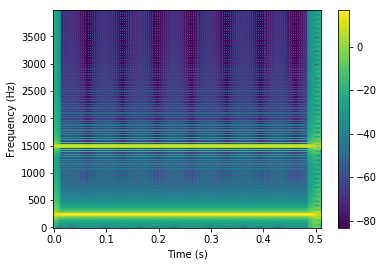
Note that the negative frequencies are not displayed since the STFT of a real signal is symetric hermitian, and that boundary effects appear at the beginning and the end of the time axis.
Reconstruction is obtained by:
In [7]:
y = istft.apply(X)
print('Reconstruction: {}'.format(y))
print('Reconstruction error: {:.3f} dB'.format(10 * np.log10(np.mean(np.abs(x - y)**2))))
Reconstruction: Waveform, fs=8000Hz, length=4000, dtype=float64, 0 missing entries (0.0%)
[ 1.5         1.17327041  0.57481454 ...,  0.26179427  0.22650352
  0.60675673]
Reconstruction error: -314.983 dB
Example on a synthetic complex signal
Create a waveform composed of two sines
In [8]:
nu1 = 1/33
nu2 = 3/16
duration = 0.5
fs = 8000
t = np.arange(0, int(duration*fs)) / fs
x = Waveform(np.exp(1j*2*np.pi*t*nu1*fs) + 0.5*np.exp(1j*2*np.pi*t*nu2*fs) , fs=fs)

print(x)
np.real(x).show_player()
Waveform, fs=8000Hz, length=4000, dtype=complex128, 0 missing entries (0.0%)
[ 1.50000000+0.j          1.17327041+0.65119101j  0.57481454+0.72521585j
 ...,  0.26179427+0.88142073j  0.22650352+0.46102256j
  0.60675673+0.44769223j]
Out[8]:
In [9]:
X = stft.apply(x)
print(X)
_ = X.plot_spectrogram(dynrange=100.)
========================
TF representation
------------------------
TF parameters
{'hop': 16, 'n_bins': 512, 'win_name': 'sine', 'win_len': 256, 'win_array': None, 'win_type': 'analysis', 'is_tight': False, 'convention': 'lp', 'param_constraint': 'pad', 'zero_pad_full_sig': False}
------------------------
Signals parameters
{'fs': 8000, 'sig_len': 4000}
------------------------
512 frequency bins
256 frames
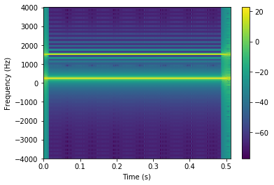
Note that all the frequencies are shown since the signal is complex.
Reconstruction is obtained by:
In [10]:
y = istft.apply(X)
print('Reconstruction: {}'.format(y))
print('Reconstruction error: {:.3f} dB'.format(10 * np.log10(np.mean(np.abs(x - y)**2))))
Reconstruction: Waveform, fs=8000Hz, length=4000, dtype=complex128, 0 missing entries (0.0%)
[ 1.50000000 +2.72299507e-17j  1.17327041 +6.51191011e-01j
  0.57481454 +7.25215846e-01j ...,  0.26179427 +8.81420728e-01j
  0.22650352 +4.61022561e-01j  0.60675673 +4.47692229e-01j]
Reconstruction error: -312.610 dB
Example on a real sound
Load test sound
In [11]:
from ltfatpy import gspi
x, fs = gspi()
x = Waveform(x, fs=fs)
Note that one may also use static method
Waveform.from_wavfile(filename) in order to load a Waveform
object from an audio file.
Apply STFT and display properties of Stft data
In [12]:
X = stft.apply(x)
print(X)
========================
TF representation
------------------------
TF parameters
{'hop': 16, 'n_bins': 512, 'win_name': 'sine', 'win_len': 256, 'win_array': None, 'win_type': 'analysis', 'is_tight': False, 'convention': 'lp', 'param_constraint': 'pad', 'zero_pad_full_sig': False}
------------------------
Signals parameters
{'fs': 44100, 'sig_len': 262144}
------------------------
257 frequency bins
16384 frames
Get a related Istft object, apply istft, display properties of reconstruction
In [13]:
y = istft.apply(X)
print('Reconstruction: {}'.format(y))
print('Reconstruction error: {:.3f} dB'.format(10 * np.log10(np.mean(np.abs(x - y)**2))))
Reconstruction: Waveform, fs=44100Hz, length=262144, dtype=float64, 0 missing entries (0.0%)
[  4.49622788e-20  -2.42328347e-20   3.05175781e-05 ...,   9.46044922e-04
   2.74658203e-03   4.05883789e-03]
Reconstruction error: -333.369 dB
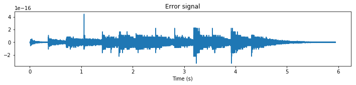
Note that x-y computes the difference between two Waveform
object and returns a new Waveform, that may be displayed or
processed, as below. Many operators can be applied in the same way to
Waveform objects.
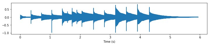
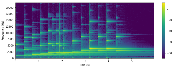
In [14]:
plt.figure(figsize=(12,2))
x.plot(y_axis_label=None)

plt.figure(figsize=(12,4))
X.plot_spectrogram(dynrange=100.)

plt.figure(figsize=(12,2))
(x-y).plot(y_axis_label=None)
plt.title('Error signal')
Out[14]:
Text(0.5,1,'Error signal')